SHORT DESCRIPTION
The Global Ocean Forecast System GOFS16 is an operational ocean analysis and forecast system that runs daily at the Euro-Mediterranean Center on Climate Change since early 2017. GOFS16 produces 7-day forecasts of the state of the global ocean and sea ice: ocean temperatures, salinities and currents, as well as sea ice thickness and concentration . The system is based on a global eddying ocean (Iovino et al. 2016), combined with a state-of-the-art data assimilation system, OceanVar (Storto et al. 2011, Storto & Masina 2016), that has been massively parallelized (Cipollone et al., 2020) and it is capable of assimilating high resolution space-borne and conventional observing networks, including hydrographic profiles and several satellite data.
SYSTEM
The GOFS16 modeling system
| NEMOv3.4 ocean configuration coupled to LIM2 (EVP) sea ice model | |
|---|---|
| Mesh: | tripolar grid [180ºW-180ºE; 78ºS-90ºN] with 1/16º (6.9 km) horizontal spacing at the equator (increasing poleward to ~2 km) and 98 vertical levels with partial step |
| Grid size: | 5762 × 3963 × 98 points |
| Bathymetry: | ETOPO2 for the deep ocean, GEBCO for the continental shelves, BEDMAP2 for Antarctica region |
| Atmospheric Forcing: | operational NCEP analyses and forecasts; bulk CORE formulation |
| Runoff: | monthly climatology from Dai et al. 2009 and Antarctic freshwater fluxes (Jacobs et al. 1992) |
The GOFS16 analysis and forecasting numerical core is based on version 3.4 of the NEMO ocean model (Madec and the NEMO team, 2012). The configuration (described in Iovino et al. 2016) is a global, eddying configuration of the ocean and sea ice system with a horizontal resolution of 1/16 degree at the Equator, corresponding to 6.9 km, that increases poleward as cosine of latitude, leading to 5762 × 3963 grid points horizontally, and roughly 3 km in the polar region. Ocean and sea ice are on the same horizontal mesh, a non-uniform tripolar grid, computed at CMCC following the semi-analytical method of Madec and Imbard (1996). The vertical coordinate system is based on fixed depth levels and consists of 98 vertical levels with a grid spacing increasing from approximately 1 m near the surface to 160 m in the deep ocean. The bathymetry is generated from three distinct topographic products: ETOPO2 (US Department of Commerce, 2006) is used for the deep ocean, GEBCO (IOC, IHO and BODC, 2003) for the continental shelves shallower than 300 m, and Bedmap2 (Fretwell et al., 2013) for the Antarctic region, south of 60◦ S. The result is modified by two passes of a uniform Shapiro filter, and finally hand editing is performed in key areas.
The ocean component OPA is a finite difference, hydrostatic, primitive equation ocean general circulation model, with a free sea surface. The NEMO code solves the primitive equations using as prognostic variables: 3D temperature, salinity, meridional and zonal velocities and 2D sea-surface height. In the current version a linearized free-surface formulation is used (Roullet and Madec, 2000) and a free-slip lateral friction condition is applied at the lateral boundaries. Tracer advection follows a total variance dissipation (TVD) scheme (Zalesak, 1979) while vertical mixing is achieved using the turbulent kinetic energy (TKE) closure scheme (Blanke and Delecluse, 1993). The model interactively computes air-surface fluxes of momentum, mass, and heat. Forcing fields are provided from NOAA operational system with 0.25 degree spatial resolution. The turbulent variables are applied at a 6 hourly frequency and radiative and freshwater fluxes are daily fields. The surface boundary conditions are computed using the bulk formulation by Large and Yeager (2004). The water balance is computed as evaporation minus precipitation and runoff. The evaporation is derived from the latent heat flux, precipitation is provided by NCEP as daily averages, while the river runoff is added at the surface as a monthly climatology (Dai and Trenberth 2002) that includes 99 major rivers and coastal runoff estimates, with a global annual discharge of ∼1.32 Sv. The ocean component is coupled to the Louvain-la-Neuve sea Ice Model (LIM2) that includes the representation of both the thermodynamic and dynamic processes. The ice dynamics are calculated according to external forcing from wind stress, ocean stress, and sea surface tilt and internal ice stresses using C grid formulation. The elastic–viscous–plastic formulation of the sea ice rheology is used.
The GOFS16 data assimilation system
OceanVar is a three-dimensional variational (3Dvar) data assimilation scheme with updates from multiple data sources. The scheme was originally developed for the Mediterranean Sea (Dobricic and Pinardi, 2008), later extended to the global ocean (Storto et al., 2011) and recently massively parallelized in a hybrid MPI-OpenMP environment to bear global high-resolution grid (Cipollone et al., 2020). The background-error covariance matrix accounts for vertical covariances (modeled through the use of multivariate EOFs) and horizontal correlations (through the application of recursive filters). Horizontal correlation length-scales have been scaled to the 1/16º mesh from the reference 1/4º resolution configuration to maximise the impact of dense satellite datasets such as SLA and SST, improving the ocean initial condition for the short-term forecast. Observation processing includes background quality checks, thinning of dense datasets, spatial (statistical) unbias for SLA and the removal of diurnal SST retrivials. In addition to the 3Dvar assimilation, GOFS16 uses a nudging scheme for surface temperature, salinity and sea ice concentration.
The assimilated data includes: Near-real-time sea level anomaly L3 observations (from Cryosat2, Jason3, Sentinel 3a and Altika satellites) provided by CMEMS; Near-real-time in-situ observations coming from moorings, Argo floats, Expand-able Bathy Termographs (XBTs), and Conductivity-Temperature-Depth (CTDs) gathered together in the CMEMS catalog; Near real time SST data: Advanced Very High-Resolution Radiometer (AVHRR) from NOAA and Advanced Microwave Scanning Radiometer 2 (AMSR2) from NASA. The analysis of GOFS16 includes a nudging scheme to correct the heat and freshwater surface fluxes using gridded SST analyses provided by NOAA (Reynolds et al., 2007) and the sea-surface salinity objective analyses from the UK MetOffice EN4 (v4.2.1), respectively. A nudging scheme to optimal-interpolation sea-ice concentration from NOAA is employed.
The GOFS16 system evaluation
The Validation/Verification process of GOFS is provided at different time scales and is performed using semi-independent analysis. The metrics refer to the “misfits” that are calculated by the data assimilation system as differences between observations and model outputs transformed at the location and time of the observations. Misfits are calculated before the data are inserted via data assimilation and can be considered as semi-independent since data are mostly sparse in time and space. The metrics are composed of:
- Root Mean Square Errors (RMSE) of temperature and salinity using misfits with ARGO-CTD and XBT (only for temperature) collected from CMEMS INS TAC. A validation webpage is available online for the analysis (https://evalid-dev.cmcc-opa.eu/evaluation/gofs/)
- RMSE of Sea Level Anomaly using misfits with satellite along track sea level anomalies from CMEMS SL TAC.
- RMSE and BIAS of Sea Surface Temperature (SST) using AVHRR and AMRS2 retrievals or AVHRR-OI.
- Daily RMSE/BIAS timeseries and spatial RMSE/BIAS maps for SST and SLA are also calculated for the first 6 days of the forecasts.
The Processing chain
The chain consists of daily production of a 6-day-long forecast, initialized by a former (daily) analysis. Each daily production (say production of day T) starts with a first integration of the sole model between T-48h and T-24h. Corrections are then calculated by the DA system and applied to a second model integration of the same day. This leads to the best initial conditions at T-24h that are used to generate the nowcast (T-24,T) and a 6-day-long forecast. The production scheme is presented in Figure 1.
The GOFS16 production consists of the following steps:
- Upstream Data Acquisition, Pre-Processing and Control of: NCEP atmospheric forcing (Numerical Weather Prediction), Satellite (SLA, SST, SIC) and in-situ (T and S) data.
- Forecast: NEMO-LIM coupled modelling system is run to produce 7-day forecast.
- Analysis: NEMO is combined with a 3DVAR assimilation scheme in order to produce the best estimation of the sea state (i.e. analysis). The NEMO +3DVAR system is run every day for 1 day into the past. The analysis provides the initial condition for the 7-day forecast.
- Post processing: the model output is made CF-compliant and transformed in different formats (binary, netcdf, etc.)
- Output Delivery.
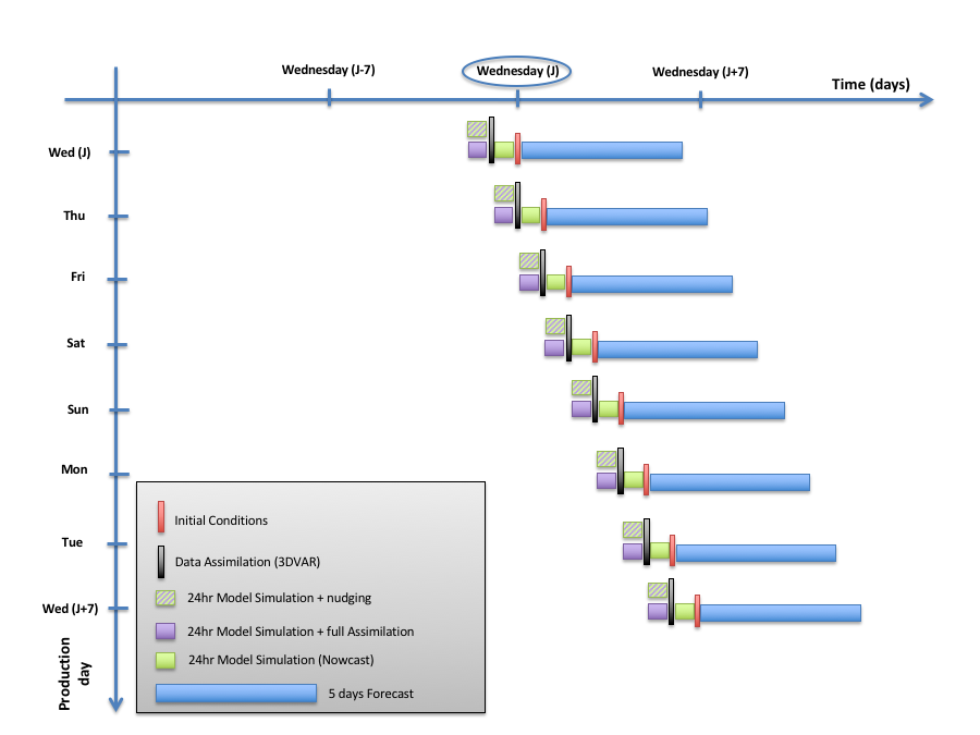
Figure 1: Production cycle scheme
Essential references
- Dai, A. and Trenberth K. E. (2002). Estimates of freshwater discharge from continents: Latitudinal and seasonal variations. J. Hydrometeor., 3, 660–687.
- Dobricic, S. and N. Pinardi (2008). An oceanographic three-dimensional variational data ssimilation scheme. Ocean Modelling, 22, 3-4, 89-105.
- Iovino, D., Masina, S., Storto, A., Cipollone, A., and Stepanov, V. N. (2016). A 1/16° eddying simulation of the global NEMO sea-ice–ocean system, Geosci. Model Dev., 9, 2665–2684, https://doi.org/10.5194/gmd-9-2665-2016.
- Madec G and the NEMO team (2012). NEMO ocean engine version 3.4. Note du Pole de la Modelisation de l’Insitut Pierre-Simon Laplace No 27 ISSN no 1288-1619.
- Reynolds, R. W., Smith T. M., Liu C., Chelton D. B., Casey K. S. and Schlax M. G. (2007). Daily high-resolution blended analyses for sea surface temperature, J. Climate, 20, 5473–5496.
- Storto, A., Dobricic, S., Masina, S., and Di Pietro, P. (2011). Assimilating along-track altimetric observations through local hydrostatic adjustments in a global ocean reanalysis system, Mon. Weather Rev., 139, 738–754.
- Storto, A., and Masina S. (2016): C-GLORSv5: an improved multipurpose global ocean eddy- permitting physical reanalysis, Earth System Science Data, 8 (2), 679–696.
- Cipollone, A., Storto A. and Masina S. (2020): “Implementing a Parallel Version of a Variational Scheme in a Global Assimilation System at Eddy-Resolving Resolution”, Journal of Atmospheric and Oceanic Technology, 37(10), 1865-1876.